This site uses CSS stylesheets.
If you can read this, your browser does not support CSS2.
Although you can still access and use the site, the pages
will not look as intended.
The basic principles of laser Doppler anemometry (LDA) are summarized here. For
a more comprehensive treatment of these principles, the reader is referred to
standard text books such as those by Durst et al. Durst76,
Durrani and Greated Durrani77, Somerscales Marton81,
Absil Absil95, and Albrecht et al. Albrecht03
Aspects of LDA that are typical for a three-component system are described in
some detail in Section
1.3.
Introduction
In LDA the Doppler-shift is determined of light scattered by a small particle
that moves with the flow. This Doppler-shift provides a measure for the velocity
of the particle, and, therefore, for the flow velocity. Since the introduction
of the technique by Yeh and Cummins Yeh the use of LDA has become
widespread in both research and industrial applications. The main advantage of
the technique over conventional measuring techniques, such as hot-wire anemometry
(HWA) and pressure probes, is that it does not require a physical probe in the
flow, i.e. it is a non-intrusive technique. Therefore, the flow is not disturbed
during a measurement. Other advantages of the technique are:
- The Doppler frequency is a measure for the velocity component in a
direction that is determined by the geometry of the optical arrangement;
- There is a linear relationship between the Doppler frequency and the velocity,
resulting in a single calibration factor. The calibration factor depends only on
the geometry of the optical arrangement and the frequency of the light source,
and is independent of the flow properties;
- The LDA combines a good spatial resolution with a high temporal resolution.
Especially for multi-component measurements, the spatial resolution of LDA is
superior to that of HWA;
- The technique is directionally sensitive which means that it is able to
measure flow reversal.
The combination of the different items makes the technique ideally suited for measurements
in turbulent flows. Both the magnitude and the direction of the instantaneous velocity
vector can be measured. It does not only give accurate information on relatively
simple statistics, such as mean velocities and Reynolds stresses, but the non-intrusive
nature also enables the measurement of more complex quantities such as spatial
correlation functions.
The list of advantages is impressive, it resembles the specification of an
ideal measuring instrument. However, it is not difficult to list some serious
drawbacks of LDA:
- LDA samples the velocity when a particle transits the measuring volume,
i.e. the region in space where the measurements are taken.
Since the particles are randomly distributed in space, the sampling times are
random as well. The random nature of the sampling process precludes the use of
many standard data-processing methods (such as the fast Fourier transform (FFT)
algorithm) for the spectral analysis of the turbulent velocity fluctuations;
- The processing of the randomly sampled data is further complicated by
the dependence of the sampling process on the flow velocity. This phenomenon is
known as the velocity bias [Tiederman]. Erroneous statistics will result if
the velocity bias is ignored during the processing of the data;
- LDA measures the velocity of small particles that move with the flow.
Since the quantity of interest is the fluid velocity, the relationship between
the particle velocity and the fluid velocity must be known.
However, the main disadvantage lies in the complexity of the measuring technique.
The complexity not only results in relatively high cost of purchasing an LDA system,
it also requires an experienced operator who is familiar with all the peculiarities
of the measuring technique.
Basic Principles of LDA
The Doppler effect forms the basis of LDA. Light scattered by a small moving particle
undergoes a shift in frequency. This frequency shift is called the Doppler frequency
and it is related to the velocity of the particle. Below, the relationship between
the Doppler frequency and the velocity is derived.
Figure 1.1 :
The light-scattering configuration.
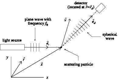 |
Consider Fig. 1.1 which shows a light source that generates a plane
light wave with frequency f0. The direction of propagation of the plane wave
is given by the unit vector  . In complex notation the plane wave is
given by
. In complex notation the plane wave is
given by
Ei( ) = Ei0e-i(2 ) = Ei0e-i(2 f0t-k0 f0t-k0  + + ), ),
|
(1.1) |
where

is the initial phase and
k0 = 2 /
/
is the wave number.
The wavelength
is related to the frequency of the light source as
= c/f0
where
c is the speed of light.
A particle passing through the plane wave scatters light in all directions and
some of the light will be received by a detector. The orientation of the detector
is determined by the unit vector

, and the detector is located at
 =
= 
.
The spherical wave emitted by the particle may be represented by [#!Adrian83!#]:
Es( - ) = - ) =  e-i(2fst-ks e-i(2fst-ks  - -  + + ), ),
|
(1.2) |
where

depends on the scattering characteristics of the particle. At the
particle
( =  )
) it follows from Eq (
1.1) and Eq (
1.2)
that
2 f0t - k0 f0t - k0 + +  = 2fst + = 2fst +  . .
|
(1.3) |
This yields the following expression for the phase

of the spherical wave
at the detector
( = )
 |
= |
2f0t + - k0 - ks  - -  |
(1.4) |
| |
= |
2f0t + - k0 - ks R - R -   t t , , |
|
where it is assumed that at time
t = 0 the distance between the particle and the
detector is
R. Furthermore,
d/dt 

is the velocity vector of the particle at
t = 0.
The frequency of the scattered light as seen by the detector,
fw, is proportional
to the time derivative of
, i.e.
2fw =  = 2f0 + = 2f0 +  (ks - k0) . (ks - k0) .
|
(1.5) |
If the velocity of the particle is small compared to the speed of light, it can
be assumed that
k0  ks
ks in Eq (
1.5), so that the frequency
of the scattered light at the detector,
fw, becomes
fw = f0 +  . .
|
(1.6) |
The second term on the right-hand side of Eq (
1.6) is known as the
Doppler frequency. It contains information on the component of the velocity in
the direction of the vector
- . This vector is determined by
the geometry of the optical arrangement of the LDA.
Heterodyne detection
It is the task of the detector to generate an output signal from which the Doppler
frequency
fD can be determined. The direct measurement of the Doppler frequency
requires a very high resolution of the detector, because the Doppler frequency
is much smaller than the frequency of light; typically
fD/f0 10-13.
In the low-velocity range, say

 < 300
< 300 m/s, the Doppler
frequency can be determined with an ``optical mixing'' or ``heterodyne'' technique
in conjunction with a square-law detector.
The essence of heterodyning is that when two light waves with slightly different
frequencies,
fw1 and
fw2, are mixed on the surface of a square-law
detector, the output signal oscillates with the difference frequency
fw1 - fw2.
Figure 1.2:
The optical arrangement for the dual-beam heterodyne LDA.
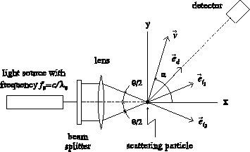 |
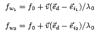
Because of its superior signal-to-noise ratio, the most widely used optical configuration
is the dual-beam heterodyne configuration. Figure 1.2 shows the optical
arrangement for the dual-beam configuration. Eq (1.6) can be applied
to both incident beams, resulting in
The unit vectors

and

indicate the direction of
the incident beams, and the Doppler frequency
fD is now defined as the difference
between
fw1 and
fw2.
Inspection of Eq (
1.7) shows that
fD is a measure for the velocity
component in the direction of
- . The Doppler frequency
is independent of the orientation of the detector with respect to the incident
beams, which enables the use of large apertures to collect more scattered light.
When a particle passes through the overlap region of the incident beams, i.e. the so-called measuring volume, it scatters light in all directions.
A square-law detector, usually a photomultiplier tube, then receives light with
two slightly different frequencies, fw1 and fw2. The relationship
between the output signal y(t) and the input signal x(t) of a photomultiplier
is given by [#!Marton81!#]
y(t) =   x(t')2dt', x(t')2dt',
|
(1.8) |
where
Ts is the time constant of the photomultiplier and the constant
S represents
the radiant sensitivity.
According to Eq (
1.5) the input signal can be written as
x(t) = a1cos(2fw1t +  ) + a2cos(2fw2t + ) + a2cos(2fw2t +  ) , ) ,
|
(1.9) |
where
 -
- 
is the phase difference between the two light waves. The
phase difference is assumed to be constant, which indicates the need for a coherent
light source such as a laser. On combining Eqs (
1.7) through (
1.9)
the following expression for the output signal of the photomultiplier is obtained
(assuming
Tsfw1  1
1 and
Tsfw2 1)
y(t) =  Sa12a22 + Sa1a2 Sa12a22 + Sa1a2 cos(2fDt + - ). cos(2fDt + - ).
|
(1.10) |
For small values of the time constant
Ts, say
Ts 10-9 s, Eq (
1.10)
reduces to the following well-known expression for the output signal of the photomultiplier
|
y(t) = Sa12a22 + Sa1a2cos(2fDt + - ).
|
(1.11) |
The first term on the equation's right-hand side is known as the pedestal; it is
the result of the spatial distribution of the light intensity in the overlap region
of both beams. The second term, called the Doppler burst, carries the desired information,
because it oscillates with the Doppler frequency
fD.
Referring to Fig.
1.2, it is easy to see that the expression for the
Doppler frequency, Eq (
1.7), can be rewritten as
where

is the angle between the unit vectors
and
,
i.e.
is the crossing angle of the incident laser beams. Furthermore,

is the angle between the velocity vector and the
x-axis.
The frequency difference
fD can be positive or negative depending on the value
of
. However, the output of the photomultiplier cannot distinguish between
positive and negative values of
fD because
cos(- fD) = cos(fD).
Figure 1.3 :
The effect of frequency shift on the relationship between the
particle velocity and the frequency of the photomultiplier output signal.
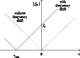 |
Figure 1.4 :
The interference of two plane light waves.
![\begin{figure}\centerline{
\epsfxsize=64mm
\epsffile[142 204 714 516]{plaatjes/fmodel.prn} }
\end{figure}](img66.png) |
As a result, the LDA in its basic form is unable to determine the sign of the
velocity. The insensitivity to the direction of the particle velocity is usually
referred to as the ``directional ambiguity.''
The common method to remove this ambiguity is frequency shifting. In that case
the frequency of one of the incident beams in Fig.
1.2 is shifted by
a constant value
fs.
This can be achieved with an acousto-optic Bragg cell. Due to the frequency
shift the relationship between Doppler frequency and particle velocity becomes
(assuming
fs  f0
f0)
fD = fs +  || sin || sin , ,
|
(1.13) |
as illustrated in Fig.
1.3. If the shift frequency
fs is chosen
larger than the Doppler frequency that corresponds to the smallest anticipated
velocity in the flow,
vmin, each value of
| fD| is uniquely related to
one velocity value, and, as a consequence, the directional ambiguity is removed.
In practice, one usually sets the shift frequency
fs about two times larger
than the Doppler frequency that corresponds to
vmin [#!Tropea86!#].
An alternative procedure to derive the relationship between the Doppler frequency
and the velocity for the dual-beam LDA, Eq (
1.12), is given by the
``fringe model,'' which is due to Rudd Rudd69. The fringe model is
often used to visualize different aspects of the dual-beam configuration, such
as the nature of the detector output signals in case the incident beams are improperly
aligned [#!Durst79!#].
It also gives an interpretation of the proportionality constant between the Doppler
frequency and the velocity in Eq (
1.12).
However, the fringe model should be considered with some reserve, because it is
incorrect in the sense that it ignores the fact that heterodyning takes place on
the surface of the photomultiplier and not at the particle, see Durst Durst82.
However, most of the predictions of the fringe model are in accordance with the
Doppler theory, as will be shown below.
If the incident beams shown in Fig. 1.4 are properly aligned, their
wavefronts are nearly plane in the overlap region, so that the light waves can
be described with Eq (1.1). The intensity of the light in the overlap
region of both beams is then given by
| I |
= |
(E10 + E20)(E10* + E20*) |
(1.14) |
| |
= |
E102 + E202 +2E10E20cos(2k0y sin( /2) + - ) , /2) + - ) , |
|
where
is the angle between the unit vectors
and
,
y is a coordinate in the direction of
-
and
- is the phase difference between the two light waves.
According to Eq (3.14) the intensity varies periodically in
y,
and the distance between two consecutive lines of constant intensity in the interference
pattern is given by
df =  . .
|
(1.15) |
The quantity
df is known as the fringe distance, and inspection of Eq (
1.12)
reveals that it is the inverse of the proportionality constant between the Doppler
frequency and the velocity. A small particle passing through the interference pattern
with a velocity component in the
y-direction of
v(= sin),
scatters light with an intensity that is proportional to the local value of
I.
The intensity of the scattered light then oscillates with frequency
It follows from a comparison with Eq (
1.12) that this is identical to
the Doppler frequency.
The fringe model can also be used to visualize the effects of applying a frequency
shift to remove the directional ambiguity. If in Fig. 1.4 the frequency
of one of the beams, say beam 1, is increased with a value fs, the intensity
of the light in the overlap region becomes
|
I = E102 + E202 +2E10E20cos(2fst + 2k0y sin(/2) + - ) .
|
(1.17) |
The fringes in the interference pattern now move with velocity
vs = dffs
in the positive
y-direction. As a result, a detector sees intensity variations
with a frequency
fs +  = fs + = fs +   sin = fD , sin = fD ,
|
(1.18) |
which is identical to Eq (
1.13), the result obtained using the Doppler
theory.
Amplitude bias
Durao and Whitelaw DurWhi79 have shown experimentally that there is a relationship
between the amplitude of a Doppler burst and the particle velocity. There study
revealed that there is a tendency for low-speed particles to produce high-amplitude
Doppler bursts, and vice versa. Through this mechanism low-velocity particles have
(on the average) a larger probability of being detected and validated by the LDA
signal processor than high-velocity particles. This bias towards low velocities
was termed ``amplitude bias'' by Durao and Whitelaw. They argued that the amplitude
bias was due to the fact that fast moving particles (on the average) spend less
time in the measuring volume than slow particles. The fast moving particles scatter
less photons and, therefore, produce Doppler bursts with smaller amplitude.
It was already shown in Section 1.2.2 (Eq (1.10)) that, in principle
at least, the amplitude A of a Doppler burst depends on the Doppler frequency
through the term
A = Sa1a2 , ,
|
(1.19) |
where
Ts is the time constant of the photomultiplier and
fD is the Doppler
frequency. Substitution of Eq (
1.18) in Eq (
1.19) yields the following expression
for
A
A = Sa1a2 , ,
|
(1.20) |
where
fs is the shift frequency,
v is the velocity component and
df is
the fringe distance. Figure
1.5 depicts the amplitude
A as a function of
v
for several values of the photomultiplier time constant
Ts ranging between
2 ns
and
32 ns. Furthermore, it is assumed that
df = 3 
m and
fs = 40 MHz.
Figure 1.5 :
The amplitude A versus the velocity v for several values
of Ts ranging between 2 ns and 32 ns.
![\begin{figure}\centerline{
\epsfxsize=68mm
\epsffile[62 74 488 473]{plaatjes/ambias.eps} }
\end{figure}](img76.png) |
Figure
1.5 shows that the amplitude
A will significantly vary with the particle
velocity only when the value of
Ts is large. Clearly, photomultipliers with
large time constants are not suited for LDA, because such photomultipliers give
rise to the amplitude bias.
Figure
1.5 also shows that the amplitude
A is practically constant for small
values of
Ts. This means that the dependence of the amplitude
A on the particle
velocity can be conveniently ignored when a so-called ``fast response'' photomultiplier
is used, which is usually the case.
The light-scattering particles form an essential element of the LDA measuring
system. In each application the suitability of the particles must be determined
in the same way as any other element of the LDA instrumentation.
In general, it is highly appreciated if the particles are cheap, easy to generate,
non-corrosive and non-toxic. However, the suitability of the particles for application
in LDA mainly depends on their dynamical and optical characteristics.
The optical characteristics should be such that the particles scatter light with
sufficient intensity for the photodetector to generate high-quality Doppler signals.
Investigations based on Mie's scattering theory, e.g. Durst Durst82,
show that the amplitude and the visibility of the Doppler signals are dependent
on the particle diameter, the refractive index of the particle material, the wavelength
of the laser light, the angle between the incident laser beams and the aperture
and orientation of the receiving optics.
Generally speaking, the amplitude and visibility of the Doppler signals increase
with increasing particle size and increasing index of refraction.
The dynamical characteristics of particles determine their ability to accurately
follow the fluctuations in the fluid velocity even at high frequencies.
The motion of a rigid, spherical particle in a viscous flow is governed by the
Basset-Boussinesq-Oseen (BBO) equation, see Somerscales Marton81.
Solutions of the BBO equation are discussed by Hjelmfelt and Mockros Hjelm66.
A simplified equation of motion is given by (see Somerscales Marton81)
where

is the fluid kinematic viscosity,
dp is the particle diameter,
up
and
uf are the particle and fluid velocities and

and

are the
particle and fluid densities, respectively.
The equation's left-hand side represents the force to accelerate the particle.
The term on the right-hand side is the drag of the particle for which Stokes' drag
law is used.
The validity of Eq (
1.21) is restricted to large values of the density
ratio
 /
/ and not too large acceleration. Furthermore,
the effects of, for example, centrifugal forces, electrostatic forces and gravity
are ignored.
Eq (1.21) will be used here to formulate a criterion for the diameter
of the particles. Following Hjelmfelt and Mockros Hjelm66 the fluid
velocity and the particle velocity are expressed in terms of Fourier components.
Substitution of
uf = ei t and
up =
t and
up =  (
( )eit
in Eq (1.21) yields the amplitude ratio || as
)eit
in Eq (1.21) yields the amplitude ratio || as
The amplitude ratio can be interpreted as a measure for the sensitivity of the
particles to changes in the fluid velocity. It is seen from Eq (
1.22)
that the particle motion is attenuated at high frequencies. The maximum diameter
of a particle that follows the velocity fluctuations up to
1 kHz,
5 kHz and
10 kHz for
|| = 0.99 can be determined from Eq (
1.22).
For a number of frequently used seed materials the thus obtained diameters are
listed in Table
1.1.
From these results it can be concluded that oil particles with a diameter of typically
1 m accurately track the velocity fluctuations in low-speed air
flows. High-speed flows generally require smaller particles, because of the energy
of the velocity fluctuations at higher frequencies.
Table 1.1 :
Maximum particle diameter for various seed materials.
|
|
The presence of a shock wave in a supersonic flow provides a further motivation
to use submicron particles.
Due to the strong decelerations across the shock wave the particle velocity lags
the fluid velocity. This phenomenon has been studied by Yanta et al. Yanta71
and more recently by Maurice Maurice92.
The particle lag may result in a severe overestimation of the mean velocity and
the turbulence intensity at locations directly downstream of the shock wave if too
large particles are used. In general, particles that accurately follow the abrupt
velocity changes in supersonic flows should have diameters less than
0.3 m.
There are flows with practical relevance for which Eq (1.21) is invalid.
In vortical flows the centrifugal forces induce a migration of particles away
from the core region (for
> 1), thus reducing the particle concentration
in the core. The particle concentration may become so low that LDA measurements
in the core become almost impossible as reported by Meyers and Hepner MeyHep88.
Details on the particle motion in vortical flows can be found in e.g. Dring and
Sou Dring78.
Signal processor
The principle task of a signal processor is to extract the Doppler frequency (i.e. velocity)
from the photomultiplier output signal. Usually, the signal processor also measures
other quantities such as the arrival time of the particles and the duration of
the Doppler bursts, i.e. the transit time of the particles.
Two commonly used signal processors for sparsely seeded flows are ``counter processors''
and ``spectrum analyzers.'' A detailed discussion of the characteristics of the
two types of processors and a comparison between their performances is beyond the
scope of this thesis. Instead, this section describes only the basic principles
of one representative of the latter type of signal processor.
The processor to be described is the Burst Spectrum Analyzer (BSA) which is manufactured
by Dantec, and available since the late 1980s.
The BSA processor performs a spectral analysis of the bandpass-filtered output
signal of the photomultiplier. The Doppler frequency then follows from the location
of the peak in the computed power spectrum.
The basic principles of the Dantec BSA are illustrated in Fig. 1.6.
Figure 1.6 :
The basic principles of the Dantec BSA processor.
![\begin{figure}\centerline{
\epsfxsize=115mm
\epsffile[22 162 836 533]{plaatjes/bsa.eps} }
\end{figure}](img96.png) |
The output signal of the photomultiplier is first amplified by a factor set by
the operator and then bandpass filtered to remove frequency components outside
the anticipated range of Doppler frequencies. A burst detection scheme determines
whether the bandpass filtered signal contains a Doppler burst or not. Burst detection
can be based on the pedestal or on the so called ``envelope.''
The envelope is obtained by rectifying and low-pass filtering of the bandpass filtered
signal. When the envelope exceeds a
25 mV threshold, the sampler and the transit
time counter are started and the arrival time is measured. The sampler is restarted
each time the envelope exceeds the next higher threshold level (
50 mV,
75 mV
etc.). This is done to ensure that the samples are taken from the central part
of the Doppler burst. The transit time counter is stopped when the envelope decreases
below
12.5 mV.
While the burst detection scheme is carried out, the bandpass filtered signal is
led through a mixer unit which shifts the power spectrum by a value of fc towards
lower frequencies. The aim of this shift is to increase the resolution of the computed
power spectrum. The centre frequency fc is selected by the operator in conjunction
with the bandwidth Bw so that the cut-off frequencies of the bandpass filter
are given by
fc Bw/2.
The down-shifted signal is low-pass filtered and then sampled at regular time intervals,
tsam. The number of samples
nrec is called the ``record
length,'' and its value can be set by the operator at 8, 16, 32 or 64.
The inverse of the time interval
tsam is called the sampling frequency
fsam. The resolution of the computed spectrum is proportional to
fsam/nrec, which reduces to
1.5Bw/nrec
because the BSA has a fixed relationship between the sampling frequency and the
bandwidth:
fsam = 1.5Bw.
A hardwired FFT processor then computes a spectrum from the samples.
Bw/2.
The down-shifted signal is low-pass filtered and then sampled at regular time intervals,
tsam. The number of samples
nrec is called the ``record
length,'' and its value can be set by the operator at 8, 16, 32 or 64.
The inverse of the time interval
tsam is called the sampling frequency
fsam. The resolution of the computed spectrum is proportional to
fsam/nrec, which reduces to
1.5Bw/nrec
because the BSA has a fixed relationship between the sampling frequency and the
bandwidth:
fsam = 1.5Bw.
A hardwired FFT processor then computes a spectrum from the samples.
In the next step a sinc function is fitted to the computed spectrum at the frequency
with the highest peak and its neighbouring frequencies. The Doppler frequency follows
as the frequency for which the sinc function achieves a maximum.
The thus determined Doppler frequency is validated by means of a comparison between
the two highest peaks in the spectrum. The Doppler frequency is validated if the
primary peak of the spectrum exceeds the secondary peak by a factor of 4 or higher.
After validation the Doppler frequency together with the arrival time (optional)
and the transit time (optional) are transferred to a computer.
Unlike, for example, TSI counter processors, the BSA processors cannot carry out
a time-coincidence test to ensure that the measured Doppler frequencies originate
from the same particle in case of a multi-component measurement. However, the time-coincidence
test can be performed in the software that is used to reduce the raw data, provided
that for each processor the arrival times of the particles are stored on disk.
Alternatively, the different BSA processors can be run in the so called ``hardware-coincident
mode.'' This mode of operation and its consequences are discussed later in this
chapter.
The Three-Component LDA
The interest of fluid-dynamics researchers for the three-component LDA (3-D LDA)
is clear, because turbulence is a three-dimensional phenomenon and in many industrial
flows even the mean flow is three-dimensional.
In its early stages of development the 3-D LDA was notorious as far as the measurement
accuracy of turbulence statistics was concerned. An increasing number of researchers
came to the conclusion that the simultaneous measurement of three velocity components
involved much more than bearing the financial burden for adding one LDA channel
to an existing two-component system.
The 3-D LDA poses a set of problems that are unique to this instrument. Meyers,
a recognized expert in the field, sketched the development of the 3-D LDA in a
paper entitled ``The Elusive Third Component'' [#!Meyers85!#]. Perhaps the title
reflects the many problems encountered during the search for the right optical
arrangement for the instrument. This section intends to discuss these problems
and their remedies, thereby resulting in the following optical arrangement for
the 3-D LDA:
- the transmitting optics are arranged such that three (nearly) orthogonal
velocity components are measured by the individual LDA channels;
- the receiving optics are configured such that only light from the
overlap region of the three measuring volumes is collected;
- the three signal processors are operated in a ``hardware-coincident mode,''
i.e. the Doppler signals are processed only when these signals show (partial)
overlap in time on all three channels, otherwise the processor is inhibited.
The discussion of the 3-D LDA will be limited to the dual-beam configuration, because
of its superior signal-to-noise ratio.
Each channel of the 3-D LDA measures the velocity component in a direction
that is determined by the orientation of the corresponding beam pair in space.
In general, these primary or colour components are non-orthogonal and they do
not coincide with one of the cartesian velocity components
u,
v or
w.
Therefore, the primary velocity components that are measured by the 3-D LDA must
be transformed into the cartesian coordinate system.
In this section the propagation of uncertainties in the primary velocities into
the cartesian velocity components is investigated. The analysis of the transformation
matrix will show that the orientation of the three beam pairs should be such that
the primary velocity components are as close to orthogonal as possible.
Figure 1.7 :
The orientation of a primary velocity component.
![\begin{figure}\centerline{
\epsfxsize=68mm
\epsffile[130 111 686 527]{plaatjes/third.prn} }\end{figure}](img98.png) |
Figure
1.7 portrays a primary velocity component
vp that is measured
by one of the LDA channels. The orientation of this velocity component in the
x, y, z-coordinate system is given by the angles
and

. A 3-D LDA
gives rise to the following set of equations:
| vg |
= |
u cos cos cos + v cossin + w sin + v cossin + w sin |
(1.23) |
| vb |
= |
u cos cos cos + v cossin + w sin + v cossin + w sin |
|
| vv |
= |
u cos cos cos + v cossin + w sin , + v cossin + w sin , |
|
where
u,
v and
w are the components of the velocity in the orthogonal coordinate
system and
vg,
vb and
vv are the primary velocity components measured
by the green, blue and violet LDA channels, respectively. If, for reasons of
simplicity, it is assumed that the blue and green channels form an orthogonal
two-component LDA (
 =
=  - /2
- /2) that senses velocity components
in the
xy-plane (
 =
=  = 0
= 0) then Eq (
1.23) reduces to
| vg |
= |
u cos + v sin |
(1.24) |
| vb |
= |
u sin - v cos |
|
| vv |
= |
u coscos + v cossin + w sin . |
|
Without loss of generality it may also be assumed that
 = /2
= /2, so that
the third component,
w, can be expressed in terms of the primary velocities as
This equation shows that the coefficients of the primary velocities become large
for small values of

. This causes the third component
w to be very
sensitive to uncertainties in the measured primary velocities caused by, for example,
calibration errors or processor inaccuracies. In case the third component is measured
directly, i.e.
= /2, this extreme sensitivity is absent. So, ideally
the transmitting optics of the 3-D LDA should be configured such that the device
senses nearly-orthogonal velocity components.
In a more detailed analysis of the coordinate transform, Morrison et al. Morris90
showed that the uncertainty propagation into the third component is even more
severe for higher-order statistics, such as the Reynolds stress
 ,
than it is for the mean velocity
,
than it is for the mean velocity
 . They conclude that the tilt angle
should be at least 30o to keep the error propagation within
reasonable limits.
This requirement on the tilt angle poses a number of practical problems. Because
many researchers do not know how to solve these problems (or are simply unaware
of the orthogonality requirement), most operational 3-D LDAs are of the non-orthogonal
type with small . The practical problems are as follows.
First, a large tilt angle requires optical access to the experimental facility
from two adjacent sides which is difficult to realize in many existing wind tunnels.
The second problem has to do with the alignment of the three beam pairs. The conventional
procedure to align the beam pairs involves either a small pinhole or a microscope
objective [#!Absil95!#].
Both methods can still be applied to the 3-D LDA as long as the tilt angle
remains small, say
< 15o, but they cannot be used for larger tilt
angles. Consequently, the orthogonal 3-D LDA requires a new alignment procedure.
. They conclude that the tilt angle
should be at least 30o to keep the error propagation within
reasonable limits.
This requirement on the tilt angle poses a number of practical problems. Because
many researchers do not know how to solve these problems (or are simply unaware
of the orthogonality requirement), most operational 3-D LDAs are of the non-orthogonal
type with small . The practical problems are as follows.
First, a large tilt angle requires optical access to the experimental facility
from two adjacent sides which is difficult to realize in many existing wind tunnels.
The second problem has to do with the alignment of the three beam pairs. The conventional
procedure to align the beam pairs involves either a small pinhole or a microscope
objective [#!Absil95!#].
Both methods can still be applied to the 3-D LDA as long as the tilt angle
remains small, say
< 15o, but they cannot be used for larger tilt
angles. Consequently, the orthogonal 3-D LDA requires a new alignment procedure.
In a study of the accuracy of a 3-D LDA, Boutier et al. Boutier85 found that some of the
measured Reynolds stresses were systematically high, due to a phenomenon that they
called ``virtual particles.'' The phenomenon is a consequence of the fact that
any 3-D LDA has at least one measuring volume that does not fully overlap the
other two. Only partial overlap of the measuring volumes can be achieved because
the different optical axes cannot all coincide in 3-D LDA.
This is in contrast to the two-component LDA where both measuring volumes usually
share a single optical axis. The typical situation for a 3-D LDA is sketched in
Fig.
1.8 where the optical axes of measuring volumes
A and
B include an angle
. One of these measuring volumes actually consists
of two fully overlapping volumes that is formed by two beam pairs (but that is not
essential here.) Assume that each measuring volume senses a velocity component that
lies in the plane spanned by the optical axes of measuring volumes
A and
B.
Figure 1.8 :
The virtual-particle phenomenon in 3-D LDA.
![\begin{figure}\centerline{
\epsfxsize=46mm
\epsffile[201 102 586 522]{plaatjes/boutier1.prn} }
\end{figure}](img117.png) |
Now consider the following ``multiple-particle'' event. Volume A measures
a particle with velocity component va at time ta whereas a particle with
velocity component vb is measured by volume B at time tb. To verify
whether the measurements on the two LDA channels stem from a single particle, it
is common to apply a simultaneity criterion. In other words: if the arrival times
ta and tb satisfy the criterion
| ta - tb| <  , where is a
user-selected time-coincidence window, then it is assumed that both measurements
stem from a single particle. The LDA subsequently produces the velocity pair (va, vb)
as if it represents the velocity components of a single particle.
However, in the case of the multiple-particle event sketched in Fig. 1.8,
the arrival times ta and tb may satisfy the simultaneity criterion, but they
do not originate from the same particle. As a result, a ``virtual particle'' with
velocity components (va, vb) is created, which will cause erroneous velocity
statistics.
, where is a
user-selected time-coincidence window, then it is assumed that both measurements
stem from a single particle. The LDA subsequently produces the velocity pair (va, vb)
as if it represents the velocity components of a single particle.
However, in the case of the multiple-particle event sketched in Fig. 1.8,
the arrival times ta and tb may satisfy the simultaneity criterion, but they
do not originate from the same particle. As a result, a ``virtual particle'' with
velocity components (va, vb) is created, which will cause erroneous velocity
statistics.
Boutier reasoned that the virtual-particle phenomenon was a complicated function
of the tilt angle , the time-coincidence window , the local flow
conditions and the seed density. However, a solution to the problem was not given.
Intuitively, it is clear that lowering the seed density will decrease the probability
that virtual particles will occur, but it will not eliminate the problem. The only
sensible way to circumvent the virtual-particle phenomenon is to collect data only
from the region in space that is common to all (three) measuring volumes, which
can be achieved by the positioning of small pinholes in front of the photomultipliers
in conjunction with a large (near 90o) off-axis light-collection angle.
This ``spatial filtering'' also happens to be the remedy for the geometry-bias problem
that will be discussed below.
Geometry bias
In an attempt to quantify the findings of Boutier's investigation, Brown Brown89
simulated the operation of a typical 3-D LDA using a Monte-Carlo approach. The
results of this study confirmed the existence of the virtual-particle phenomenon,
and showed that, as expected, the probability of a virtual-particle occurrence
increases with increasing seed density.
Recall from the previous section that the virtual particles were able to pass the
simultaneity criterion, thereby causing erroneous velocity statistics. Brown's
study showed that even without virtual particles, which was easy to realize in
the simulation, the velocity statistics as measured by the 3-D LDA were in error.
As a result, the study revealed a previously unidentified error source. This error
was termed the ``geometry bias,'' and it is a direct result of the 3-D LDA measuring-volume
geometry in conjunction with the concept of a time-coincidence window.
Figure 1.9 :
The geometry bias in 3-D LDA.
![\begin{figure}\centerline{
\epsfxsize=45mm
\epsffile[218 79 603 527]{plaatjes/brown1.prn} }
\end{figure}](img119.png) |
Figure
1.9 depicts the measuring-volume geometry that was used in Brown's study.
The geometry is identical to that shown in Fig.
1.8 for a tilt angle
= 60o.
Consider particle
a that passes through the overlap region of the measuring
volumes. For simplicity it is assumed that its velocity component in the
y-direction
is zero. Clearly, this particle will satisfy the time-coincidence criterion
regardless of the magnitude of the velocity components
u and
w. This is not
the case for particles
b and
c which do not pass through the overlap region.
Particle
b is assumed to have zero
w-component and it will satisfy
the time-coincidence criterion only if the in-plane velocity component
u is
sufficiently large. Particle
c is supposed to have a non-zero
w-component
and it cannot pass the time-coincidence test if the
w-component is large
compared to the
u-component, simply because it will not arrive at the other measuring
volume. This illustrates that the 3-D LDA measuring-volume geometry in combination
with the time-coincidence window will cause a bias towards high in-plane velocity
components and small out-of-plane velocity components.
The time-coincidence concept, which works very satisfactorily for a conventional
two-component LDA, is inadequate for the 3-D LDA.
To circumvent the geometry bias, Brown Brown89 suggested a new mode of operation for
the LDA signal processors known as the ``channel-blanking mode'' or the ``hardware-coincident
mode.''
In this mode of operation each signal processor will process a Doppler burst only
when Doppler bursts are also present on the other two channels, in the sense that
the three Doppler bursts (partially) overlap in time. If this is not the case,
the signal processors are inhibited. Due to the hardware-coincident mode, data
will be acquired only from the overlap region of the three measuring volumes, so
that particle a will be measured by the 3-D LDA while particles b and
c are ignored1.1.
The hardware-coincident mode removes the geometry bias, which is a single-particle
event. But it does not eliminate the virtual-particle phenomenon, because this
is a multiple-particle event. To eliminate both error sources, the 3-D LDA
requires both the channel-blanking mode and the collection of scattered light
from the overlap region only, as mentioned in the previous section. The beneficial
effect of these measures is that the spatial resolution of the 3-D LDA is high
compared to that of a conventional two-component LDA. The latter is usually operated
in the (off-axis) forward-scatter or backward-scatter mode, resulting in a sensitive
region with relatively large dimensions.
The sensitive region for the 3-D LDA is reduced to the overlap region of the three
measuring volumes. This more-or-less spherical region has a characteristic length
equal to the diameter of the individual measuring volumes which is typically 10
times smaller than the length of the measuring volumes. On the other hand, the
smaller measuring volume of the 3-D LDA will result in a much lower mean data rate
as compared to the two-component LDA for the same seed density.

![\begin{figure}\centerline{
\epsfxsize=31mm
\epsffile[289 85 556 530]{plaatjes/brown2.prn} }
\end{figure}](img120.png)
 .
.
 with
with